In the part 1 of this project, I described how to train a deep learning model to identify species of mammals present in a photo. This could be an useful functionality, for example, in the cellphone of wildlife enthusiasts. Now, how can we create a more complete application, one that goes beyond tracing boxes around the identified mammals and actually feeds back interesting information to the user?
An obvious first choice would be to rely on existing expert filled databases available online, such as Map of Life, Mammal Diversity Database or the IUCN Red List of Threatened Species. This would be a reliable, complete and readily-available solution… but boring! I wanted a more challenging and generalizable solution! What if we wanted to find information not present in these databases? So I decided to experiment with a sort of version of the wisdom of the crowds concept applied to internet published content. My intutition was: if I collect a large enough number of web pages related to a specific mammal, I can statistically estimate the countries where it is most likely to be found by counting the frequency of occurrence of countries names in those pages.
This corpus-based solution will definitely not, for this example, be as reliable as hand-filled, domain expert-based solution. However, the unsupervised nature of the method makes it, at least in principle, generalizable to other tasks (e.g. what does this species like to eat?) and scalable to larger numbers of classes (e.g. it gets cheaper than the expert-based solution if we would do it for all known species). Furthermore, it will be an interesting exercise for creative problem solving! Let’s go ahead then, this project will involve the following steps:
- Find relevant webpages and scrape their content
- Run Named Entity Recognition to find countries names
- Create appealing visualizations
1. Web scraping
How to gather so many web pages with information about the mammal species? No one better than Mr. know-it-all Google to give it a hand! But now, how to do it automatically, without the need of a sapiens mammal clicking work? I used the handy MarioVilas’ googlesearch to get me the first 200 google results to entries such as “giraffe animal countries”. Keep in mind that automated querying is against Google’s Terms of Service and abusing it might get your IP banned, so be polite! The amount of links we’re gathering here is small and we only need to make it once, so keep the limit of one request per minute and you will be (hopefully) safe.
To install the python packages is as easy as pip install google. Here’s an usage example that will create a CSV file with all the page links for every mammal:
from googlesearch import search, get_random_user_agent
import pandas as pd
import time

mammal_list = [ 'hedgehog', 'lion', 'wolf', 'fox', 'zebra', 'giraffe',
                'bat', 'sloth', 'capybara', 'elephant', 'rhino',
                'hippo', 'tiger', 'panda', 'kangaroo', 'koala' ]

df = pd.DataFrame(data=mammal_list, columns=['species'])
df['countries_search'] = ''
df['countries_search'] = df['countries_search'].astype(object)

#Search 100 Google results for each species
for mammal in mammal_list:
    all_urls = []
    results = search(mammal+" animal habitat", num=50, stop=200, pause=60.,
                     only_standard=True, user_agent=get_random_user_agent())
    [all_urls.append(i) for i in results]

    df.at[df['species']==mammal,'countries_search'] = [all_urls]
    df.to_csv('mammals_websites.csv', index=False)
    time.sleep(60)
The next step is to retrieve the text content from each one of these pages. To scrape this large set of links, we’ll used Scrapy. Scrapy has a bit steepy learning curve, but it really comes at hand for small projects such as this, once you learn the basics of it! Here’s a nice tutorial for it. To install Scrapy, just run pip install scrapy.
Now we want to create the spiders, which are objects that Scrapy will use to navigate through web pages and retrive information from them. The following code creates a spider class find_countries that will open the urls in the list start_urls relative to the species mammal, will extract all text content inside the html p tags, remove some of the html content from the text and save the results in TXT files:
import os
import scrapy
from scrapy.crawler import CrawlerProcess

class find_countries(scrapy.Spider):
    name = "find_countries_for"
    def __init__(self, mammal, start_urls, *args, **kwargs):
        self.mammal = mammal
        self.start_urls = start_urls
        super(find_countries, self).__init__(*args, **kwargs)

    def parse(self, response):
        paragraphs = response.xpath('//p[.//text()]').extract()
        aux = response.url.replace(".","").replace(":","").replace("/","")+'.txt'
        fname = os.path.join('mammals_raw_txt', self.mammal, aux)
        dirname = os.path.dirname(fname)
        if not os.path.exists(dirname):
            os.makedirs(dirname)
        with open(fname, "w", encoding="utf-8", errors="ignore") as text_file:
            for item in paragraphs:
                item = item.replace("<"," ").replace(">"," ").replace("/"," ")
                text_file.write("%s\n" % item)


#dataframe containing websites to search for
df = pd.read_csv('mammals_websites.csv')

mammal_list = ['hedgehog', 'lion', 'wolf', 'fox', 'zebra', 'giraffe', 'bat',
               'sloth', 'capybara', 'elephant', 'rhino', 'hippo', 'tiger',
               'panda', 'kangaroo', 'koala']

process = CrawlerProcess()

#Iterate over all mammal species
for mammal in mammal_list:
    aux0 = df.loc[df['species']==mammal,'countries_search']
    aux1 = aux0.values.tolist()[0]
    full_list = aux1.strip("[]").replace("'", "").split(", ")
    list_urls = []
    for url in full_list:   #excludes youtube links
        if "youtube" not in url:
            list_urls.append(url)

    #set-up crawler
    process.crawl(find_countries, mammal=mammal, start_urls=list_urls)

process.start()
This should create one folder per mammal species, with one TXT file per web page scraped containing mostly the text content of those pages. Our raw database is now ready to be used offline, with whatever the world wide web has to say about kangaroos and sloths!
2. Named Entity Recognition
With the corpus at hand, we move on to extract meaningful information: the whereabouts of those mammals. Now, how to find countries names in this sea of texts? The simplest way to do so would be to sweep the whole article strings looking for exact matches with each existent country’s name. Simple and possibly accurate… but boring and possibly slow! Instead, I decided to use the super cool SpaCy library available for python, it has many ready to use Natural Language Processing (NLP) functionalities and works really fast.
To install Spacy, just do pip install -U spacy. You will also need to download the language model to be used for inference, that’s as simples as python -m spacy download en. I got the best results with the large model but, if it is excessively large for your application, you can use medium or small models.
The task we need to solve is Named Entity Recognition (NER), which consists on classification of words into specific categories. SpaCy NER is able to identify a relatively wide span of object classes, amongst which GPE (Geopolitical Entity), which encompasses countries, cities and states. That’s how the code looks like:
import spacy
import os
import operator
import pandas as pd

# loads large english model
nlp = spacy.load('en_core_web_lg')

mammal_list = ['hedgehog', 'lion', 'wolf', 'fox', 'zebra', 'giraffe',
               'bat', 'sloth', 'capybara', 'elephant', 'rhino', 'hippo',
               'tiger', 'panda', 'kangaroo', 'koala']

df = pd.DataFrame(data=mammal_list, columns=['species'])
df['country_counts'] = ''
df['country_counts'] = df['country_counts'].astype(object)
df['number_results'] = 0

for mammal in mammal_list:
    all_files = os.listdir(os.path.join('mammals_raw_txt', mammal))
    all_sets = []
    for fname in all_files:   #all scraped pages in .txt files
        file_path = os.path.join('mammals_raw_txt', mammal, fname)
        with open(file_path, 'r', encoding="utf-8", errors="ignore") as myfile:
            data = myfile.read().replace('\n',' ').replace('type',' ').replace('=',' ')
        data = data[0:50000]   #protect from memory error
        doc = nlp(data)

        curr_ents = []
        for X in doc.ents:  #find words of a specific entity
            if X.label_ == 'GPE':
                ent_txt = (X.text).lower()
                curr_ents.append(ent_txt)

        #Gets unique values in lists
        myset = set(curr_ents)
        all_sets = all_sets + list(myset)

    #Counts number of occurrences
    wrd_cnt = {}
    for wrd in all_sets:
        if wrd not in wrd_cnt:
            wrd_cnt[wrd] = 1
        else: wrd_cnt[wrd] += 1

    #Sorts by number of occurrences
    sorted_x = sorted(wrd_cnt.items(), key=operator.itemgetter(1), reverse=True)
    df.at[df['species']==mammal,'country_counts'] = [sorted_x]

    #Number of scraped files
    df.at[df['species']==mammal,'number_results'] = len(all_files)

    df.to_csv('mammals_country_counts.csv', index=False)
We must have now a single CSV file with lists of countries names, sorted by number of occurrences in web pages associated with each mammal species. Congratulations! You just used a series of machine learning models to produce a meaningful dataset!
3. Visualization
It’s now time to explore our dataset visually on a Jupyter notebook. To create beautiful and interactive graphics, let’s use Plotly. To install it, just run pip install plotly.
In the file mammals_country_counts.csv we will find a list of unique GPE entity type counts for each mammal species. We can narrow down our scope to names of countries (and exclude regions, cities and other categories) by comparing this list with a list of know country names save in the 'countries_names.csv file. Open a notebook instance on your working environment and let’s set up a function to read the counts file and return the names and values in a clean format:
import numpy as np
import pandas as pd
import ast
import csv

def mammals_countries(mammal):
    #Load and prepare data
    df = pd.read_csv('mammals_country_counts.csv')
    npages = df.loc[df['species']==mammal]['number_results'].values[0]
    aux = df.loc[df['species']==mammal]['country_counts'].values[0]
    aux = aux.strip('[]')
    aux_all = list(ast.literal_eval(aux))

    #Check if it's a valid country name and counts occurrences
    with open('countries_names.csv', 'r') as f:
        reader = csv.reader(f)
        valid_countries = list(reader)[0]
    country_names = []
    country_counts = []
    for i in aux_all:
        if i[0].title() in valid_countries:
            country_names.append(i[0].title())
            country_counts.append(i[1])
    country_names = np.array(country_names)
    country_counts = 100*np.array(country_counts)/npages

    return country_names, country_counts
Now let’s make a function to create a bar plots with the frequencies of occurrence for each country, as a percentage of the number of pages scraped. Set Plotly to work in the notebook mode, call the mammals_countries() function to load the data, format the layout and use iplot(fig) to print it on the notebook or plot(fig, filename) to save the plot as an HTML file.
from plotly import tools
import plotly.plotly as py
import plotly.graph_objs as go
from plotly.offline import iplot, init_notebook_mode

init_notebook_mode(connected=True)

def bar_graph_mammals(mammal, cnt_threshold=5):
    #Get countries counts
    country_names, country_counts = mammals_countries(mammal)
    if len(country_names) > 30:
        country_names = country_names[0:30]
        country_counts = country_counts[0:30]

    #Make Plotly graphics
    trace0 = go.Bar(
        x=country_names,
        y=country_counts,
        marker=dict( color='rgb(158,202,225)',
                     line=dict(color='rgb(8,48,107)', width=1.5) ),
        opacity=0.6 )

    data = [trace0]

    layout = dict( height=370, width=900, xaxis=dict(tickangle=-45), title=mammal+' presence',
                   yaxis=dict( title='Occurrences on web pages [%]' ),
                   paper_bgcolor='rgba(0,0,0,0)',
                   plot_bgcolor='rgba(0,0,0,0)',
                   shapes=[{
                        'type': 'line',
                        'x0': 0,
                        'y0': cnt_threshold,
                        'x1': len(country_names),
                        'y1': cnt_threshold,
                        'line': {
                            'color': 'rgb(0, 0, 0)',
                            'width': 1,
                            'dash': 'dot'}}] )

    fig = go.Figure(data=data, layout=layout)

    #Display bar plots
    iplot(fig)

    #Save bar plots
    plot(fig, filename='media/bar_graph_'+mammal+'.html')

    return country_names, country_counts


mammal = 'tiger'
cnt_threshold = 10
country_names, country_counts = bar_graph_mammals(mammal, cnt_threshold=cnt_threshold)
Let’s check the results (click on a mammal):
Bat Capybara Elephant Fox Giraffe Hedgehog Hippo Kangaroo Koala Lion Panda Rhino Sloth Tiger Wolf Zebra
Since we scraped all the google search results indiscriminately, some spurious results will happen (e.g. tigers in Barbados), but they will most likely have low counts and a simple threshold (e.g. 10%) might be enough to get rid of most of this noise.
What’s better than a nice graphic to tell a story, right? I’ll tell you what: a map! Next step we will create an informative map related to each mammal species. A good map style for that is the choropleth, which paints each geographical region with different color intensities. Creating interactive and beautiful maps is very easy with the Folium library for python. To install it, run pip install folium. Now, in our notebook:
import folium

# function to generate map plots
def map_mammals(mammal, cnt_threshold, country_names, country_counts):
    # make an empty map
    my_map = folium.Map(location=[20, 0], tiles="Mapbox Bright", zoom_start=2)
    #my_map = folium.Map(location=[20, 0], tiles="Stamen Terrain", zoom_start=2)

    #Countries layer
    countries_geo = 'world-countries.json'
    countries_df = pd.read_json(countries_geo)
    for index, row in countries_df.iterrows():
        countries_df.at[index,'country'] = row['features']['properties']['name']

    chosen_indexes = country_counts > cnt_threshold
    chosen_data = pd.DataFrame(data=country_names[chosen_indexes], columns=['country'])
    chosen_data['quantity'] = country_counts[chosen_indexes]

    # Add the color for the chloropleth
    folium.Choropleth(
        geo_data=countries_geo,
        name='choropleth',
        data=chosen_data,
        columns=['country', 'quantity'],
        key_on='properties.name', #'feature.id',
        fill_color='OrRd',
        fill_opacity=0.7,
        line_opacity=0.2,
        nan_fill_color ='#ffffff00',
        legend_name='Estimated presence of '+mammal+'s',
    ).add_to(my_map)

    #create mammal markers and add them to map object
    centroids = pd.read_csv('centroids.csv')  #centroid marks to print icons
    for index, row in chosen_data.iterrows():
        #create icons from images
        icon = folium.features.CustomIcon('./icons/icon_'+mammal+'.png', icon_size=(25,25))
        #create popup descriptions
        popupIcon = "<strong>mammal</strong><br>Population"
        if sum(centroids['country']==row.country) == 1:
            lat = centroids.loc[centroids['country']==row.country]['lat']
            lng = centroids.loc[centroids['country']==row.country]['lng']
            folium.Marker([lat.values[0],lng.values[0]], tooltip=mammal, popup=popupIcon, icon=icon).add_to(my_map)

    # Save to html
    my_map.save('media/map_'+mammal+'.html')

    return my_map

mammal = 'tiger'
cnt_threshold = 10
my_map = map_mammals(mammal, cnt_threshold=cnt_threshold, country_names=country_names, country_counts=country_counts)
my_map
Let’s check the results (click on a mammal):
Bat Capybara Elephant Fox Giraffe Hedgehog Hippo Kangaroo Koala Lion Panda Rhino Sloth Tiger Wolf Zebra
The cute mammal icons were taken from Flaticon, they get positioned at the calculated centroids for each country that hits the minimum threshold. And that’s it! We finished the visualization for the unsupervised data mining stage of the project. If we look carefully, we will obeserve that the results are not 100% accurate, but most of the times they get pretty close to what we would expect to see in terms of species distributions by regions of the world. In the next part, we will create a web application that joins the object identification functionality from the last session to the data mining and visualization results of this session.
Tip: Both Plotly and Folium make it easy to create beautiful visuals and export directly to html. After producing your superb HTML graphics and maps, here’s a great tool to render them as a vector PDF, if you need to use them as static figures.
4. Limitations, errors and what I learned from them
Having your application indicating that giraffes live in Ecuador can be disappointing, but errors are not always so bad. We can learn form them! Here’s a couple of interesting things I learned from the limitations of this project:
-
This was an interesting implementation of the wisdom of the crowds principle applied to web pages, but not without shortcomings. The first limitation is intrinsic to the world wide web: a disproportionally large chunk of the whole web content is produced in the United States, making it likely that the name “United States” will appear more often than others by chance. Making the search exclusively in english reinforces this bias.
-
The method works well for niche specific species (kangaroos, zebras, sloths) but gets innacurate for widespread species (bats, foxes, hedgehogs), most likely due to the limited sample size of web pages and the language bias.
-
Because of zoos, certain countries might have their names appearing regularly together with some species, even if those species are not natural from those countries.
-
Hippos in Colombia, wtf?? Yes, they were brought in the 80s by Pablo Escobar for his personal zoo and now are roaming by the country.
-
Sloths in India?? That’s a typical result of our search for species being too unspecific. Sloth bears inhabits the southern Asia region and are more badasses than the Latin American sloths (like, tiger-ass-kicking level badass)
-
Australia scored significantly high in 15 of these 16 species! Or Australia has the most diverse zoos in the world, or it’s definitely the weirdest fauna in the globe.
5. References and resources
- Map of Life
- Mammal Diversity Database
- IUCN Red List of Threatened Species
- Wisdom of the crowds
- Corpus-Based Knowledge Representation
- MarioVilas’ googlesearch
- Google’s Terms of Service
- Scrapy
- Scrapy tutorial
- SpaCy
- SpaCy language models
- Named Entity Recognition
- Jupyter notebook
- Plotly
- Folium
- Cute icons from Flaticon
- HTML to PDF conversion tool
- Hippos in Colombia
- Badass sloth bear