The Cool Mammals Project

GitHub page for this project

Largely due to its demonstrated power in the field of computer vision, the interest in multilayer (deep) neural networks has boomed during the current decade, as reflected in the massive investments from big tech companies and the development of ever more efficient and complex models. In fact, the cutting edge architectures increased so much in size that one would give up altogether the plans of training those models if not in possession of expensive hardware configurations. Fortunately, together with the technical advances, we have been observing growing efforts in democratizing the access and usage of these models by means of open sourcing codes and transfer learning.

Transfer learning refers to the technical possibility of using complex networks that have been already trained in huge, general data sets (computationally heavy), and just fine tune some parts of it to a specific task (computationally light). This concept is specially useful if we are interested in advanced object detection models. Lucky for us, the freely available TensorFlow Object Detection API provides several pre-trained models and allows for fine tune training to new custom classes.

“Now, what should I use these amazing tools for? Well, of course, to identify cool mammals around the world!”. So I set up my mission to detect 16 species of cool mammals using an object detection model. There are many detailed and comprehensive tutorials available on how to set up the TensorFlow Object Detection API, out of which I’d recommend this, this and this. I’ve encountered, however, some problems not covered by these and, since I’m using a software for annotation different from theirs, I thought it would be good to document the step-by-step of my project as well. Setting up a custom object detection application will require the following steps:

Install required software (python modules, repositories and other dependences)
Form the training and test datasets (download and annotate the images, convert the files)
Fine tune a pre-trained model
Export the updated graph and deploy model for inference

1. Installing modules

Although not necessary, I highly recommend using Anaconda to manage your python environments and modules installation (you can also use pip command inside a conda environment). Here’s a list of commands to first create a new environment and then install all necessary modules for this project:

$ conda create -n your_env_name pip python=3.7
$ conda activate your_env_name
$ conda install -c anaconda cython
$ conda install -c anaconda contextlib2
$ conda install -c anaconda pillow
$ conda install -c anaconda lxml
$ conda install -c anaconda jupyter 
$ conda install -c conda-forge opencv
$ conda install -c conda-forge matplotlib
$ pip install tensorflow

The next step is cloning the git repository for TensorFlow models, installing and compiling Protobuf and installing the COCO API. Follow the instructions here.

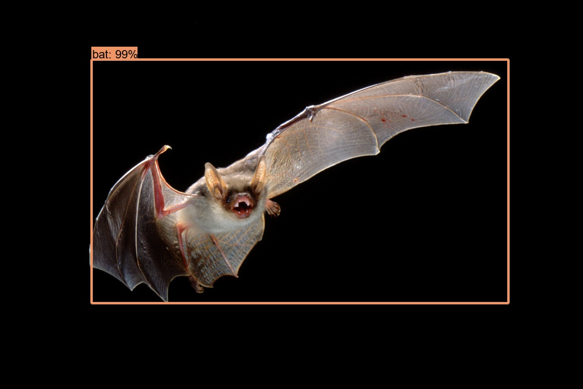
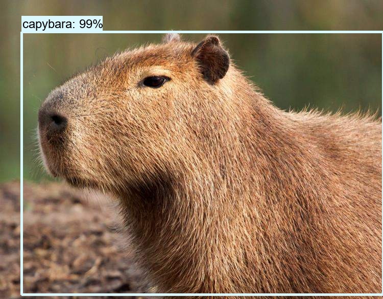
Once all modules are successfully installed, let’s play with the object_detection_tutorial.ipynb on Jupyter notebook and check how the pre-trained model performs on pictures of mammals we’re interested in. This tutorial is found at models/research/object_detection, inside the cloned TensorFlow models repository. You can add any JPG photos you want to the test_images\ folder for inference and also try it with any pre-trained models form the Model Zoo.

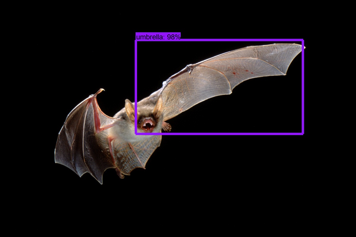
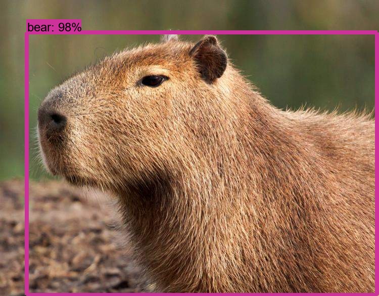
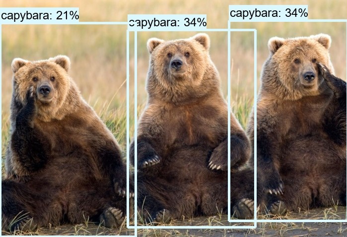
Oh ohh! Capybaras are classified as bears, which couldn’t be farther form the truth (they’re the most chilled animals ever), and we certainly wouldn’t like our robots to grab us a bat once it starts raining… now, if we want to avoid rabies from bat bites and unnecessary alarms to escape from capybaras, we would like to fine tune this model to learn those species properly. Let’s move on to define our classes, download photos of them and annotate the examples.

2. Data acquisition and annotation

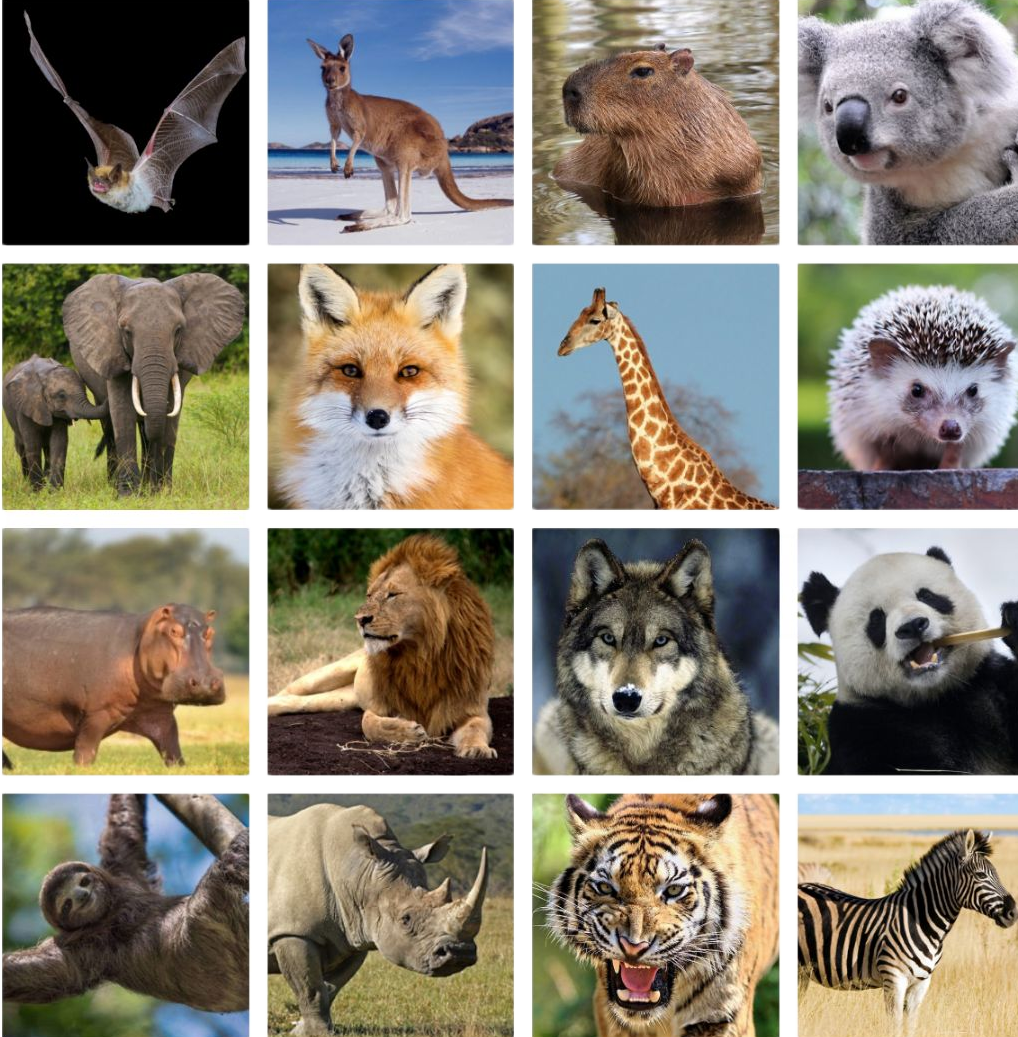
A list of 16 cool mammals was chosen to form the training set. Of course this is not an extensive account of all known mammal species and the ones lacking in the list will probably be classified as a similar another, e.g. porcupines (not in the trained set) will likely be classified as a hedgehogs (present in the trained set! Also, check this fantastic russian animation from 1975). For each of the 16 chosen species, we perform a google images search (make sure to filter for only JPG and minimum size of 240x240) and use the Fatkun Batch Download Image chrome extension to download 100 examples for training and 10 examples for testing.

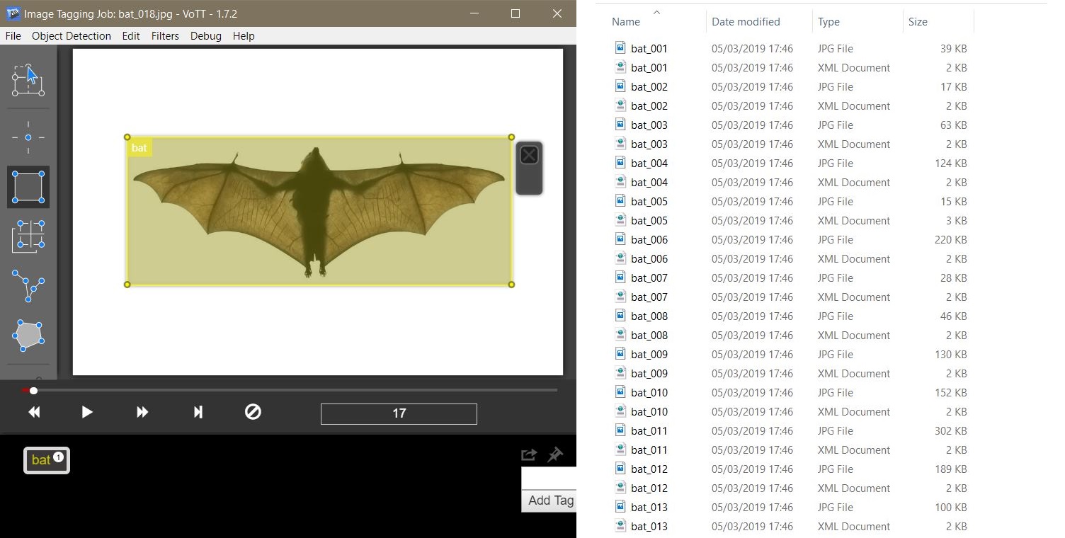
Some of the coolest mammals ever! Wonder if I can teach a robot to identify them...

There are many good annotation tools available. Personally, I like to use VOTT, it’s an easy to use annotation tool that exports to several data formats and can be coupled to a pre-trained object recognition API to semi-automatize the tagging process of big datasets. After annotating all examples for the training and test sets, go to Object Detection → Export Tags, choose the export format to Tensorflow Pascal VOC and export it to a new folder of your choice. Inside this new folder you will find the subfolder Annotations, that’s where all the XML annotations are saved, and the subfolder JPEGImages, that’s where VOTT made copies of your images, probably for organization purposes. Check if the number of annotations match the number of copied images and copy all images and annotations to the same folder. VOTT will also export a label_map.pbtxt file, which contains a dictionary mapping each mammal class to an integer number.

We still have two steps ahead: 1) convert the XML annotations to a CSV file and 2) convert the CSV files to Tensorflow RECORDS files. A guide on how to organize the folders and files for this project can be found on the GitHub page for this project, which is inspired by this video tutorial. Here’s an illustration of the annotation tool and the initial organization of JPG and XML files:

(left) Annotation example. (right) .jpg and .xml files organization.

For the step 1, we’re gonna download this script and modify it in a couple of places. First, the files must be assigned together with their extension, so go ahead and change the xml_to_csv() function, on the first line of the value variable, to value = (root.find('filename').text+'.jpg'. Second, four lines below, the texts need first to be transformed to float and then to int, change it e.g. int(float(member[4][0].text)). Third, inside the main() function, choose the correct image_path to where the annotations and images are and change the filename for the generated CSV file. Run the script for both train and test sets, we should now have two CSV files (one for train and one for test).

For the step 2, we’re gonna download this script and again modify it a bit. This function imports the module dataset_util which sits at /models/research/object_detection in the cloned tensorflow repository, so go ahead and add it to your path by adding sys.path.append("../models/research"). Finally, in the function class_text_to_int() we must enter the label classes and assign an integer number to each one of them, for example:

def class_text_to_int(row_label):
    if row_label == 'wolf':
        return 1
    elif row_label == 'zebra':
        return 2
    elif row_label == 'sloth':
        return 3
...        

Make sure the return integers match the labels as found at the PBTXT file generated by VOTT when you saved the annotations. Run the generate_tfrecord.py file as follows, substituting the paths according to your own folders organization:

python generate_tfrecord.py --csv_input=data\train_labels.csv --output_path=data\train.record --image_dir=images\train
python generate_tfrecord.py --csv_input=data\test_labels.csv --output_path=data\test.record --image_dir=images\test

and the files test.record and train.record should be created. The dataset is ready, now let’s move on to train the model!

Tip: Annotating can be a tedious and long job, so it is useful to resume the task at other times or to break it up in sessions for few classes each time. In the latter case, for every export VOTT will create a different label_map.pbtxt containing only the classes you tagged for. No problem, you can always edit this file yourself, just make sure to match the class/integer pairs in it to the pairs you wrote on the generate_tfrecord.py file.

3. Model training – transfer learning

First, download the ssd_inception_v2_coco model from the Model Zoo and extract it’s contents in the pre-trained subfolder inside your project’s main folder. Next, download the configuration file for the same model here. Edit the configuration file as described here and save it at the subfolder training. Finally, copy the file models/research/object_detection/legacy/train.py to your project’s main folder.

Everything should be ready for training the model now. Run the following command from your project’s main folder, substituting the path names as necessary:

python train.py --logtostderr --train_dir=training/ --pipeline_config_path=training/ssd_inception_v2_coco.config

If everything is working fine, you should start seeing a series of prints like INFO:tensorflow:global step 1234: loss = 1.234 (1.234 sec/step). Congratulations! You got your transfer learning running. If you run into error No module named 'nets', a pair of solutions can be found here.

To keep track visually of the training session, use TensorBoard. Open a new Anaconda prompt, activate your project’s environment, go to the project’s main folder and run:

tensorboard --logdir=data/ --host localhost --port 8088

This will run the TensorBoard server locally on your machine. Open your browser and navigate to http://localhost:8088, you should now be able to see the evolution of the training session. If you run into error ValueError: Invalid format string, the solution can be found here.

Now the training might take a while, specially if you’re not making use of fancy GPUs. Let it run until you observe a plateau at lower values. Acceptable values for the Loss that I’ve seen people suggesting are usually around 1. Once you decide it’s time to stop training, hit CTRL+C on the training prompt and go check the training subfolder, it should contain a pair of checkpoint models (big files), with numeric values representing the step at which those were saved.

Tip: TensorFlow automatically saves the training sessions every couple of minutes, and you can stop and resume the training session from any check point. Start with larger values for the learning rate for rapid convergence and, whenever your training gets stuck fluctuating around a value, change it to smaller values in the pipeline.xml file.

4. Export and use the model

Now it’s time to export the fine-tuned model to be used for inference. Copy the file models/research/object_detection/export_inference_graph.py to your project’s main folder, choose the model checkpoint model.ckpt-XXXX you’d like to use (probably the last one) and, in the Anaconda prompt, enter:

python export_inference_graph.py --input_type image_tensor --pipeline_config_path training/ssd_inception_v2_coco.config --trained_checkpoint_prefix training/model.ckpt-XXXX --output_directory trained-inference-graphs/output_inference_graph_v1.pb

Ta-da! Habemus model! Check the newly created subfolder trained-inference-graphs/ and observe that it is similar to the subfolder we downloaded for the pre-trained ssd_inception_v2_coco in the first part. They both have the same model architecture, we have just adapted the weights at the last layers to detect our custom objects (cool mammals in that case)!

Now let’s copy the object_detection_tutorial.ipynb, the notebook we used before, to your project’s main folder and modify it to use our newly trained model. Just change the PATH_TO_FROZEN_GRAPH, PATH_TO_LABELS and PATH_TO_TEST_IMAGES_DIR to match the paths of, respectively, the newly exported model, the new classes PBTXT file and your test images (NOT the training ones). Let’s check how it performs:

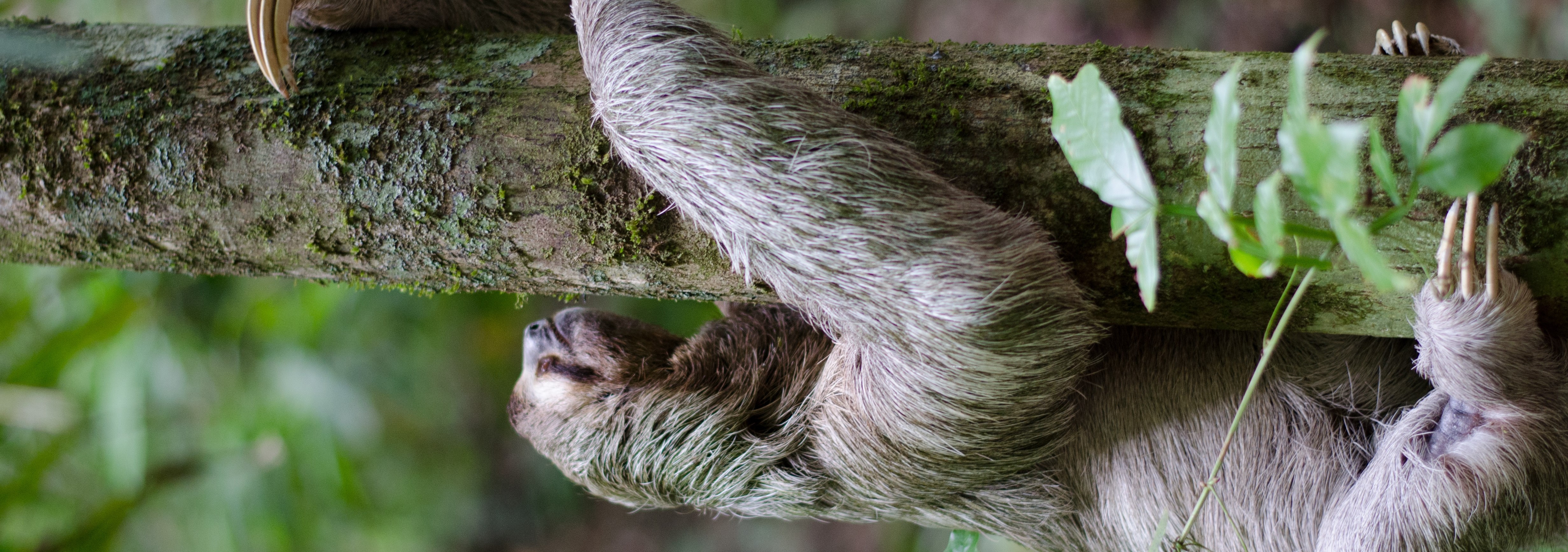
Success! No risk of our nature-explorer robot to miss out bats or capyabaras anymore! The fine-tuned SSD Inception achieved over 85% accuracy in my test dataset, which sounds good! However, as important as knowing where we’re good at, is to know where we fail. An immediate limitation is the small range of mammals that we trained the model to recognize. Here’s an example of an EPIC fail:

5. Limitations, errors and what I learned from them

Except for being eaten by bears, not every fail is a doom, though. We can learn form them! Here’s a couple of interesting things I learned from the limitations of this project:

100 examples per class might be too little if you have similar classes, such as fox and wolf or bear and capybaras. For data driven utilities, the more, the better.
Sometimes the Object Detection model classifies bats as foxes. Well, guess what? In many parts of the world bats are colloquially named flying foxes! One of these places is the Pemba Island, in the coast of Tanzania, that has it’s own flying fox species. That makes sense, some bats really look like foxes in their faces.

6. References and resources

Twitter Facebook Google+ LinkedIn

The Cool Mammals Project